Friends,
So far we have discussed about various Excel functions for example VLOOKUP, HLOOKUP, IF, SUMIF, COUNTIF etc, we discussed about conditional formatting, how to find duplicate or unique values, we used tools like filter & sort etc., and now in this article we will discuss about PIVOT TABLE - which is a very easy and excellent tool provided by Microsoft Excel to summarize a very large data.
There is lot of things in Pivot Table which can help you in many ways to prepare your data for analysis. This tool in Excel has many customization options to facilitate the data analysis. Proper use of Pivot Table in Excel can reduce the time taken to prepare a report to view or to analyze.
Pivot table is a tool which can summarize large data. We
use Pivot Table in Excel to get customized summary from a large or bulky data. Pivot table
summaries data by combining the duplicate figures into one unique figure or
data. Pivot Table appears to be a very complicated tool in Excel for some people but it is not that complicated if you understand the functions of its various parts. Creating
a Pivot Table is very simple, understand your requirement and plan accordingly before inserting Pivot Table.
There are few rules which you have to follow to insert a pivot table, these are
listed below.
1.
You need an organized data, here 'organized'
means, there should not be any blank column or rows in a Table of data
2. Each Column must have a column header or column name.
2. Each Column must have a column header or column name.
3.
No merged column header should present
in the column header or within the data
How to Create or Insert a Pivot Table
1.
Select a cell within your data.
2.
Go to Insert Tab, in Tables sub-menu
click PivotTable
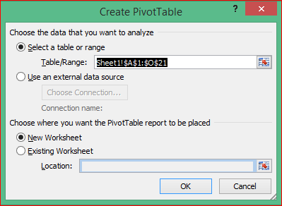
 |
| Create PivotTable Window |
 |
| Insert PivotTable Table Option |
3. A small window will appear "Create PivotTable" as shown above, you can notice that there is four radio buttons, of which the first one is 'Select a Table or Range' and this option is automatically detects the data range. Check this data range, if it is not OK select it.
4. In the next block you can notice there is another two radio buttons below the first one, New Worksheet and Existing Worksheet. Click OK if you want to insert PivotTable in new Excel Sheet in the same Workbook or you may select the next radio button and provide the destination cell in the same Excel Sheet. Click OK, I always use New Worksheet.
5. Now you will see a Blank format in the Excel sheet and at the extreme right one small tool window named PivotTable Field List - this is the column selection window and your PivotTable design will depend upon this arrangement and therefore, it is very important. Now please watch carefully the below snapshot.
 |
| PivotTable Field List Window |
6.
This PivotTable filed chooser window
has few parts (bordered by red), four small boxes, you need to understand the function of these
boxes. We will start from the data part for the ease of understanding.
a) Values : In the extreme right and
in the bottom of PivotTable Field List window
you will find a little box named as Values, here you need to put the data part i.e.,
data column e.g., Sales Target, or Sales value etc., you can put one or more than
one fields or columns by either ticking column headers displayed in 'Choose
fields to add to report' or you can Drag & Drop the columns in this
box.
b)
Row Labels : In left of the Values box there is another small box named as Row Labels, you need to put that column
for which you need the data, e.g., Zone, Employee Name, Employee code etc., remember
this is not your data part. You will get summarized data respective to this
field, for example, North Zone -> 50 (Target), as shown in the bellow picture.
 |
| Basic PivotTable |
We
have just created a basic Pivot Table in Excel. Now let us understand the functions
of another two boxes namely Report
Filter & Column Labels
c) Report Filter : Now let suppose
in my data I need to derive employee wise performance or Target but one by one Employee
Code. Here we can use Report Filter, the box located above the Row Labels box.
Just Drag & Drop Employee Code in this box and you are done. You will now
see a new entry in the top of the Pivot Table as Employee Code (All), with a
drop down list. You can select any item in this drop down list and the related
data will be displayed in the Pivot Table hiding all other data.
Please
refer to the below image.
 |
| Use of Report Filter in Pivot Table |
d) Column Labels : Now let suppose I
need the data date wise, date will be column header and the Target value will
be date wise & day wise. Here we need to put the date column in Column
Labels, as shown in the below picture.
 |
| Use of Column Labels in Pivot Table |
This is the basic methods to use PivotTable in Microsoft Excel. Hope you have fully understand the functions of four magical boxes in Pivot Table. If you have any problem in this part please post in comment box and in my next article I will show you some amazing techniques in Pivot Table in advanced level, till then keep reading...
Thank
you...
No comments:
Post a Comment